DataFrame基础入门笔记

PythonPandas库中,DataFrame是一个二维的标签化数据结构,可以看作是表格型数据结构,其中每个列可以是不同的数据类型(数字、字符串、布尔值等),并且每列都有一个标签或名称。

Series相比,DataFrame提供了更多的功能和灵活性,可以用来处理和分析更复杂的数据集。例如,可以使用列名来访问或修改数据,进行各种数据清洗和转换操作,或者进行基于多个列的数值计算。

DataFrame是一个表格型的数据结构,含有一组有序的列。DataFrame可以被看做是由Series组成的字典并且共用一个索引。

创建方式

创建方式有很多种,如下:

1
2
3
4
5
6
7
8
9
10
11
12
13
14
15
16
17
18
19
20
21
22
23
24
25
26
27
28
29
30
31
32
33
34
35
36
# 使用字典创建
In [161]: pd.DataFrame({"x":[1, 2, 3, 4], "y":[5, 6, 7, 8]}, index=['a', 'b', 'c', 'd'])
Out[161]:
x y
a 1 5
b 2 6
c 3 7
d 4 8

# 使用series
In [163]: pd.DataFrame({'x':pd.Series([1, 2, 3], index=['a', 'b', 'c']), 'y':pd.Series([4, 5, 6, 7], index=['b', 'c','d','a'])})
Out[163]:
x y
a 1.0 7
b 2.0 4
c 3.0 5
d NaN 6

# 使用多维数组(列表)创建,且不指定行/列索引
In [166]: pd.DataFrame(np.random.randint(1, 20, 15).reshape((3, 5)))
Out[166]:
0 1 2 3 4
0 6 18 17 8 13
1 3 12 14 14 13
2 6 19 15 3 3

# 使用多维数组(列表)创建,指定行/列索引
In [169]: pd.DataFrame([[6,18,17, 8,13],
...: [3,12,14,14,13],
...: [6,19,15, 3, 3]]
...: , index=['x', 'y', 'z'], columns=['a', 'b', 'c', 'd', 'e'])
Out[169]:
a b c d e
x 6 18 17 8 13
y 3 12 14 14 13
z 6 19 15 3 3

其实说白了,只要是符合DataFrame的二维数组(列表)形式,都可以作为DataFrame的数据源

1
2
3
4
5
6
7
8
9
10
11
12
13
14
15
# 三维数组
In [174]: np.random.randint(1, 20, 18).reshape((2, 3, 3))
Out[174]:
array([[[10, 14, 3],
[14, 4, 1],
[ 8, 7, 6]],

[[16, 3, 7],
[ 3, 8, 19],
[ 7, 19, 13]]])

# 使用三维数组创建DataFrame直接报错了
In [175]: pd.DataFrame(np.random.randint(1, 20, 18).reshape((2, 3, 3)))
---------------------------------------------------------------------------
ValueError: Must pass 2-d input. shape=(2, 3, 3)

但是实际开发中,我们的数据源很少使用上述形式读取进来,更多的是通过文件、sql

这里简单通过一个csv文件做个示例,事实上pd读取文件不止csv,还有excel/json/xml等等

1
2
3
4
5
6
7
8
9
10
11
12
13
14
15
# 查看data.csv文件内容
In [7]: ! cat data.csv
a,b,c
1,11,111
2,22,222
3,33,333

# 读取data.csv文件
In [8]: pd.read_csv('data.csv')
Out[8]:
a b c
0 1 11 111
1 2 22 222
2 3 33 333

写示例

1
2
3
4
5
6
7
8
9
10
11
12
13
14
15
16
17
18
19
20
21
22
23
24
25
26
27
28
29
30
31
32
33
34
35
36
37
In [21]: df1
Out[21]:
a b c
0 1 11 111
1 2 22 222
2 3 33 333

In [22]: df2
Out[22]:
a b c
0 111 222 333
1 112 223 334
2 113 224 335
3 114 225 336

# df運算
In [23]: df = df1-df2

In [24]: df
Out[24]:
a b c
0 -110.0 -211.0 -222.0
1 -110.0 -201.0 -112.0
2 -110.0 -191.0 -2.0
3 NaN NaN NaN

# 保存数据
In [25]: df.to_csv('data1.csv')

# 查看文件内容
In [26]: ! cat data1.csv
,a,b,c
0,-110.0,-211.0,-222.0
1,-110.0,-201.0,-112.0
2,-110.0,-191.0,-2.0
3,,,

常用属性

index

获取索引

1
2
3
4
5
6
7
8
9
10
11
12
13
In [33]: df =pd.DataFrame(np.random.randint(1, 20, 6).reshape((3, 2)), index=['x', 'y', 'z'], columns=['a', 'b'])

In [34]: df
Out[34]:
a b
x 7 10
y 3 18
z 13 2

In [35]: df.index
Out[35]: Index(['x', 'y', 'z'], dtype='object')


T

转置

1
2
3
4
5
6
7
8
9
10
11
12
In [36]: df
Out[36]:
a b
x 7 10
y 3 18
z 13 2

In [37]: df.T
Out[37]:
x y z
a 7 3 13

columns

获取列索引

1
2
3
4
5
6
7
8
9
10
In [39]: df
Out[39]:
a b
x 7 10
y 3 18
z 13 2

In [40]: df.columns
Out[40]: Index(['a', 'b'], dtype='object')

values

获取值数组

1
2
3
4
5
6
7
8
9
10
11
12
13
In [42]: df
Out[42]:
a b
x 7 10
y 3 18
z 13 2

In [43]: df.values
Out[43]:
array([[ 7, 10],
[ 3, 18],
[13, 2]])

describe()

获取快速统计

1
2
3
4
5
6
7
8
9
10
11
12
13
14
15
16
17
18
19
In [45]: df
Out[45]:
a b
x 7 10
y 3 18
z 13 2

# 获取每列统计信息
In [46]: df.describe()
Out[46]:
a b
count 3.000000 3.0
mean 7.666667 10.0
std 5.033223 8.0
min 3.000000 2.0
25% 5.000000 6.0
50% 7.000000 10.0
75% 10.000000 14.0
max 13.000000 18.0

索引和切片

DataFrame是一个二维数据类型,所以有行索引和列索引。

DataFrame同样可以通过标签和位置两种方法进行索引和切片

loc属性和iloc属性.

使用方法: 逗号隔开,前面是行索引,后面是列索引

行/列索引部分可以是常规索引、切片、布尔值索引、花式索引任意搭配

1
2
3
4
5
6
7
8
9
10
11
12
13
14
15
16
17
18
19
20
21
22
23
24
25
26
27
28
29
30
31
32
33
34
35
36
37
38
39
40
41
42
43
44
45
46
47
48
49
50
51
52
53
54
55
56
57
58
59
60
61
62
63
64
65
66
67
68
69
70
71
72
73
74
75
76
77
78
79
80
81
82
83
84
85
86
87
88
89
90
91
92
93
94
95
96
97
98
99
100
101
102
103
104
105
106
107
108
109
In [57]: df
Out[57]:
a b
x 7 10
y 3 18
z 13 2

# 使用嵌套索引方式为先列后行
In [58]: df['a']['x']
Out[58]: 7

# 获取b列
In [59]: df['b']
Out[59]:
x 10
y 18
z 2
Name: b, dtype: int32

# 使用loc/iloc方式为先行后列
# 获取x行,所有列
In [61]: df.loc['x']
Out[61]:
a 7
b 10
Name: x, dtype: int32

# 获取x行,所有列
In [62]: df.loc['x',]
Out[62]:
a 7
b 10
Name: x, dtype: int32

# 获取x行,所有列
In [63]: df.loc['x',:]
Out[63]:
a 7
b 10
Name: x, dtype: int32

# 获取所有行,b列
In [69]: df.b
Out[69]:
x 10
y 18
z 2
Name: b, dtype: int32

# 获取所有行,b列
In [71]: df.loc[:,'b']
Out[71]:
x 10
y 18
z 2
Name: b, dtype: int32

# 获取y行,a列
In [64]: df.loc['y', 'a']
Out[64]: 3

# 获取数字索引为2行,和数字索引为1的列
In [67]: df.iloc[2, 1]
Out[67]: 2

# 获取x/z行,b列
In [77]: df.loc[['x', 'z'], 'b']
Out[77]:
x 10
z 2
Name: b, dtype: int32

# 切片,获取x到y行,a列
In [78]: df.loc['x':'y', 'a']
Out[78]:
x 7
y 3
Name: a, dtype: int32

# 获取a列大于3的行
In [88]: df[df['a']>3]
Out[88]:
a b
x 7 10
z 13 2

In [104]: df
Out[104]:
name age gender score
0 Tom 18 male 85
1 Jack 19 male 92
2 Marry 20 female 98
3 Lily 21 female 89

# 获取大于18岁,且分数在90分以上的行和列
In [105]: df[(df['age']>18) & (df['score']>90)]
Out[105]:
name age gender score
1 Jack 19 male 92
2 Marry 20 female 98

# 获取大于18岁,且分数在90分以上的所有行;仅显示name和gender列
In [106]: df.loc[(df['age']>18) & (df['score']>90), ['name', 'gender']]
Out[106]:
name gender
1 Jack male
2 Marry female


数据对齐和缺失数据

DataFrame对象在运算时,同样会进行数据对齐,其行索引和列索引分别对齐

1
2
3
4
5
6
7
8
9
10
11
12
13
14
15
16
17
18
19
20
21
22
23
24
25
26
27
In [109]: df1 = pd.DataFrame({'one':[2, 3, 5, 6], 'two':[2, 5, 9, 3]}, index=['a', 'b', 'c', 'd'])

In [110]: df2 = pd.DataFrame({'one':[1, 2, 3, 4], 'two':[5, 6, np.nan, 8]}, index=['b', 'a', 'd', 'c'])

In [111]: df1
Out[111]:
one two
a 2 2
b 3 5
c 5 9
d 6 3

In [112]: df2
Out[112]:
one two
b 1 5.0
a 2 6.0
d 3 NaN
c 4 8.0

In [113]: df1+df2
Out[113]:
one two
a 4 8.0
b 4 10.0
c 9 17.0
d 9 NaN

DataFrame处理缺失数据的相关方法
dropna(axis=0,where='any'....

1
2
3
4
5
6
7
8
9
10
11
12
13
14
15
16
17
18
19
20
21
22
23
24
25
26
27
28
29
30
31
32
33
In [119]: df
Out[119]:
one two
a 4 8.0
b 4 10.0
c 9 17.0
d 9 NaN

# 删除缺失值(默认删除整行)
In [120]: df.dropna()
Out[120]:
one two
a 4 8.0
b 4 10.0
c 9 17.0

# 删除有缺失值的行(删除整行,axis=0代表行;axis=1代表列)
In [121]: df.dropna(axis=0)
Out[121]:
one two
a 4 8.0
b 4 10.0
c 9 17.0

# 删除有缺失值的列
In [122]: df.dropna(axis=1)
Out[122]:
one
a 4
b 4
c 9
d 9

假如我们只删除一行中所有列都是NaN的行呢

1
2
3
4
5
6
7
8
9
10
11
12
13
14
15
16
17
18
19
20
21
22
23
24
25
26
27
In [124]: df.loc['e'] = [np.nan, np.nan]

In [125]: df
Out[125]:
one two
a 4.0 8.0
b 4.0 10.0
c 9.0 17.0
d 9.0 NaN
e NaN NaN

# how参数默认为any,只要有nan就删除整行或整列
In [127]: df.dropna(axis=0, how='any')
Out[127]:
one two
a 4.0 8.0
b 4.0 10.0
c 9.0 17.0

# 删除整行为nan的数据
In [126]: df.dropna(axis=0, how='all')
Out[126]:
one two
a 4.0 8.0
b 4.0 10.0
c 9.0 17.0
d 9.0 NaN

fillna()

1
2
3
4
5
6
7
8
9
10
11
12
13
14
15
16
In [115]: df
Out[115]:
one two
a 4 8.0
b 4 10.0
c 9 17.0
d 9 NaN

In [116]: df.fillna(999)
Out[116]:
one two
a 4 8.0
b 4 10.0
c 9 17.0
d 9 999.0

isnull()

1
2
3
4
5
6
7
8
9
10
11
12
13
14
15
16
17
18
In [128]: df
Out[128]:
one two
a 4.0 8.0
b 4.0 10.0
c 9.0 17.0
d 9.0 NaN
e NaN NaN

In [129]: df.isnull()
Out[129]:
one two
a False False
b False False
c False False
d False True
e True True

notnull()

1
2
3
4
5
6
7
8
9
10
11
12
13
14
15
16
17
18
19
20
21
22
23
24
25
26
27
In [132]: df
Out[132]:
one two
a 4.0 8.0
b 4.0 10.0
c 9.0 17.0
d 9.0 NaN
e NaN NaN

In [133]: df.notnull()
Out[133]:
one two
a True True
b True True
c True True
d True False
e False False

# 获取one列不为空的所有数据
In [135]: df[df['one'].notnull()]
Out[135]:
one two
a 4.0 8.0
b 4.0 10.0
c 9.0 17.0
d 9.0 NaN

常用方法

默认nan不参与计算

mean(axis=0,skipna=False)

对列 (行) 求平均值

1
2
3
4
5
6
7
8
9
10
11
12
13
14
15
16
17
18
19
20
21
22
23
24
25
26
27
28
29
30
31
32
33
34
35
36
37
38
39
40
41
42
43
In [142]: df
Out[142]:
x y z
a 4 27.0 23
b 42 39.0 43
c 30 13.0 42
d 46 32.0 47
e 49 NaN 26

# 默认按列求平均值
In [143]: df.mean()
Out[143]:
x 34.20
y 27.75
z 36.20
dtype: float64

# 指定按列求平均值
In [144]: df.mean(axis=0)
Out[144]:
x 34.20
y 27.75
z 36.20
dtype: float64

# 指定按行求平均值
In [146]: df.mean(axis=1)
Out[146]:
a 18.000000
b 41.333333
c 28.333333
d 41.666667
e 37.500000
dtype: float64

# 默认按列求平均值且nan参与计算
In [147]: df.mean(skipna=False)
Out[147]:
x 34.2
y NaN
z 36.2
dtype: float64

sum(axis=1)

对列 (行) 求和

1
2
3
4
5
6
7
8
9
10
11
12
13
14
15
16
17
18
19
20
21
22
23
24
25
26
27
28
29
30
31
32
33
34
35
36
37
38
39
40
41
42
43
In [150]: df
Out[150]:
x y z
a 2 7.0 1
b 4 9.0 7
c 4 1.0 4
d 9 9.0 6
e 8 NaN 1

# 默认按列求和
In [151]: df.sum()
Out[151]:
x 27.0
y 26.0
z 19.0
dtype: float64

# 指定按列求和
In [152]: df.sum(axis=0)
Out[152]:
x 27.0
y 26.0
z 19.0
dtype: float64

# 默认按行求和
In [153]: df.sum(axis=1)
Out[153]:
a 10.0
b 20.0
c 9.0
d 24.0
e 9.0
dtype: float64

# 默认按列求和,nan参与计算
In [154]: df.sum(skipna=False)
Out[154]:
x 27.0
y NaN
z 19.0
dtype: float64

sort_index(axis, ..., ascending)

对列 (行) 索引排序

1
2
3
4
5
6
7
8
9
10
11
12
13
14
15
16
17
18
19
20
21
22
23
24
25
26
27
28
29
30
31
32
33
34
35
36
37
38
39
40
41
42
43
44
45
46
47
48
49
In [155]: df
Out[155]:
x y z
a 2 7.0 1
b 4 9.0 7
c 4 1.0 4
d 9 9.0 6
e 8 NaN 1

# 默认按行索引默认升序
In [156]: df.sort_index()
Out[156]:
x y z
a 2 7.0 1
b 4 9.0 7
c 4 1.0 4
d 9 9.0 6
e 8 NaN 1

# 默认按行索引指定降序
In [157]: df.sort_index(ascending=False)
Out[157]:
x y z
e 8 NaN 1
d 9 9.0 6
c 4 1.0 4
b 4 9.0 7
a 2 7.0 1

# 指定按列索引默认升序
In [158]: df.sort_index(axis=1)
Out[158]:
x y z
a 2 7.0 1
b 4 9.0 7
c 4 1.0 4
d 9 9.0 6
e 8 NaN 1

# 指定按列索引指定降序
In [159]: df.sort_index(axis=1, ascending=False)
Out[159]:
z y x
a 1 7.0 2
b 7 9.0 4
c 4 1.0 4
d 6 9.0 9
e 1 NaN 8

sort_values(by, axis, ascending)

按某一列 (行) 的值排序

1
2
3
4
5
6
7
8
9
10
11
12
13
14
15
16
17
18
19
20
21
22
23
24
25
26
27
28
29
30
31
32
33
34
35
36
37
38
39
40
41
42
43
44
45
46
47
48
49
In [160]: df
Out[160]:
x y z
a 2 7.0 1
b 4 9.0 7
c 4 1.0 4
d 9 9.0 6
e 8 NaN 1

# 默认按列排序指定按x列进行默认升序排序
In [161]: df.sort_values(by='x')
Out[161]:
x y z
a 2 7.0 1
b 4 9.0 7
c 4 1.0 4
e 8 NaN 1
d 9 9.0 6

# 默认按列排序指定按x和y列进行默认升序排序
In [162]: df.sort_values(by=['x', 'y'])
Out[162]:
x y z
a 2 7.0 1
c 4 1.0 4
b 4 9.0 7
e 8 NaN 1
d 9 9.0 6

# 默认按列排序指定按x列进行指定升序、y列降序排列
In [166]: df.sort_values(by=['x', 'y'], ascending=[True, False])
Out[166]:
x y z
a 2 7.0 1
b 4 9.0 7
c 4 1.0 4
e 8 NaN 1
d 9 9.0 6

# 指定按行排序指定按a行进行默认升序排序
In [168]: df.sort_values(by='a', axis=1)
Out[168]:
z x y
a 1 2 7.0
b 7 4 9.0
c 4 4 1.0
d 6 9 9.0
e 1 8 NaN

apply(func,axis=0)

将自定义函数应用在各行或者各列上func可返回标量或者Series

1
2
3
4
5
6
7
8
9
10
11
12
13
14
15
16
17
18
19
20
21
22
23
24
25
26
27
28
29
30
31
32
33
34
35
36
37
38
39
40
41
42
43
44
45
46
47
48
49
50
51
52
53
54
55
56
57
In [169]: df
Out[169]:
x y z
a 2 7.0 1
b 4 9.0 7
c 4 1.0 4
d 9 9.0 6
e 8 NaN 1

# 对每个元素平方根操作
In [170]: df.apply(np.sqrt)
Out[170]:
x y z
a 1.414214 2.645751 1.000000
b 2.000000 3.000000 2.645751
c 2.000000 1.000000 2.000000
d 3.000000 3.000000 2.449490
e 2.828427 NaN 1.000000


# 对每个元素平方操作(自定义函数)
In [172]: df.apply(lambda x:x*x)
Out[172]:
x y z
a 4 49.0 1
b 16 81.0 49
c 16 1.0 16
d 81 81.0 36
e 64 NaN 1

# 默认df按列求和
In [176]: df.apply(np.sum)
Out[176]:
x 27.0
y 26.0
z 19.0
dtype: float64

# 指定行列求和
In [177]: df.apply(np.sum, axis=0)
Out[177]:
x 27.0
y 26.0
z 19.0
dtype: float64

# 指定按行求和
In [178]: df.apply(np.sum, axis=1)
Out[178]:
a 10.0
b 20.0
c 9.0
d 24.0
e 9.0
dtype: float64


NumPy的通用函数同样适用于pandas

时间对象

时间序列类型

  • 时间戳: 特定时刻
  • 固定时期: 如2017年7月
  • 时间间隔: 起始时间-结束时间

Python标准库处理时间对象: datetime

datetime日常大家都在用,这里不再细说了

灵活处理时间对象: dateutil

  • dateutil.parser.parse()

dateutil模块是由Gustavo Niemeyer在2003年编写而成的对日期时间操作的第三方模块

dateutil模块对Python内置的datetime模块进行扩展时区和解析

dateutil库主要有两个模块:parser和rrule,其中parser可以将字符串解析成datetime,而rrule则是根据定义的规则来生成datetime

dateutil模块特点:

  • 能够计算日期时间相对增量,例如下周、下个月、明年、每月的最后一周等
  • 可以计算两个给定日期和/或日期时间对象之间的相对增量
  • 支持多种时区格式文件的解析,例如UTC时区、TZ时区等
  • 支持包括RFC字符串或其他任何字符串格式的通用日期时间解析

安装

1
pip install python-dateutil

Dateutil库常用模块

dateutil库常用模块有三个:parser、rrule和relativedelta

1
2
3
4
from dateutil import parser, rrule, relativedelta
# dateutil.parser:将字符串解析成datetime
# dateutil.rrule:将参数输出datetime.datetime格式的时间
# dateutil.relativedelta:日期时间偏移量

parser

parser用于将字符串解析成datetime,字符串可以很随意,可以用日期时间的英文单词,可以用横线、逗号、空格等做分隔符

1
2
3
4
'''
parser.parse(str)
- str:字符串
'''

parser使用示例如下:

1
2
3
4
5
6
7
8
9
10
11
12
13
14
15
16
17
18
19
20
21
22
23
24
25
26
27
28
29
30
31
32
# 没指定时间默认0点,没指定日期默认当天,没指定年份默认当年
# 当年份放在前面时,只能按年月日的顺序
print(parser.parse('2023-11-29')) # 2023-11-29 00:00:00
print(parser.parse('10:45:52')) # 2023-11-29 10:45:52
print(parser.parse('20231129')) # 2023-11-29 00:00:00
print(parser.parse('2023.11.29')) # 2023-11-29 00:00:00
print(parser.parse('2023/11/29')) # 2023-11-29 00:00:00

# fuzzy:开启模糊匹配,过滤无法识别的时间日期字符
print(parser.parse('Today is 11-29 10:45, I feel good.', fuzzy=True)) # 2023-11-29 10:45:00

# 当只有月日时,parser会将分隔符前面的数字解析为月份,后面的为日
# 当有年份时,在前面的月份超出范围时,会自动判断哪个是月哪个是日
# 11.29解析结果异常,11-29、11/29可正常解析
print(parser.parse('11-29')) # 2023-11-29 00:00:00
print(parser.parse('11/29/2023')) # 2023-11-29 00:00:00

# 当前面的月份超过12时,parser会自动识别月和日
print(parser.parse('29/11/2023')) # 2023-11-29 00:00:00

# 当分隔符为逗号时,只有月日时,要把月放在后面
# 当分隔符为逗号时,有年份时,年份要放在后面,要把月放在前面
print(parser.parse('29,11')) # 2023-11-29 00:00:00
print(parser.parse('11,29,2023')) # 2023-11-29 00:00:00

# 识别英文的月、日
print(parser.parse('November 29')) # 2023-11-29 00:00:00
print(parser.parse('November 1st')) # 2023-11-01 00:00:00
print(parser.parse('November 29 2023')) # 2023-11-29 00:00:00
print(parser.parse('2023 November29')) # 2023-11-29 00:00:00
print(parser.parse('11:45 AM')) # 2023-11-29 11:45:00

rrule

rrule用于将字符串解析成datetime

1
2
3
4
5
6
7
8
9
10
11
12
13
14
15
16
17
18
'''
rrule.rrule(freq,dtstart,interval,wkst,count,until,by)
- freq:单位,可选的值为YEARLY、MONTHLY、WEEKLY、DAILY、HOURLY、MINUTELY、SECONDLY,即年月日周时分秒
- dtstart、until:开始和结束时间,时间格式datetime.datatime类型
- interval:间隔
- wkst:周开始时间
- count:生产时间的个数
- by:指定匹配的周期,例如,byweekday=(MO,TU):只有周一周二的匹配,取值如下:
- bysetpos:必须为整数或者整数序列,设置匹配的周期频率
- bymonth:设置匹配的月份
- bymonthday:设置匹配每月的日期
- byyearday:设置匹配每年的天数
- byweekno:设置匹配第几周
- byweekday:MO,TU,WE,TH,FR,SA,SU
- byhour:设置匹配小时
- byminute:设置匹配分钟
- bysecond:设置匹配秒数
'''

rrule使用示例如下:

1
2
3
4
5
6
7
8
9
10
11
12
13
14
15
16
17
18
19
20
21
22
23
24
25
26
27
28
29
30
31
32
33
34
35
# 生成一个连续的日期列表
print(list(rrule.rrule(rrule.DAILY, dtstart=parser.parse('2023-11-29'), until=parser.parse('2023-12-3'))))
'''
[datetime.datetime(2023, 11, 29, 0, 0), datetime.datetime(2023, 11, 30, 0, 0), datetime.datetime(2023, 12, 1, 0, 0), datetime.datetime(2023, 12, 2, 0, 0), datetime.datetime(2023, 12, 3, 0, 0)]
'''

# 间隔一天
print(list(rrule.rrule(rrule.DAILY, interval=2, dtstart=parser.parse('2023-11-29'), until=parser.parse('2023-12-3'))))
'''
[datetime.datetime(2023, 11, 29, 0, 0), datetime.datetime(2023, 12, 1, 0, 0), datetime.datetime(2023, 12, 3, 0, 0)]
'''

# 只保留前3个元素
print(list(rrule.rrule(rrule.DAILY, count=3, dtstart=parser.parse('2023-11-29'), until=parser.parse('2023-12-3'))))
'''
[datetime.datetime(2023, 11, 29, 0, 0), datetime.datetime(2023, 11, 30, 0, 0), datetime.datetime(2023, 12, 1, 0, 0)]
'''

# 只取周六和周日日期时间
print(list(rrule.rrule(rrule.DAILY, byweekday=(rrule.SA, rrule.SU), dtstart=parser.parse('2023-11-29'), until=parser.parse('2023-12-3'))))
'''
[datetime.datetime(2023, 12, 2, 0, 0), datetime.datetime(2023, 12, 3, 0, 0)]
'''

# 以月为间隔,生成3个月
print(list(rrule.rrule(rrule.MONTHLY, count=3, dtstart=parser.parse('2023-11-01'))))
'''
[datetime.datetime(2023, 11, 1, 0, 0), datetime.datetime(2023, 12, 1, 0, 0), datetime.datetime(2024, 1, 1, 0, 0)]
'''

# rrule计算日期时间差
# rrule可计算出两个datetime对象间相差的年月日等时间数量
print(rrule.rrule(rrule.DAILY, dtstart=parser.parse('20231129'), until=parser.parse('20231203')).count()) # 5
# 不足N个月的,按N个月计算;不满整月的,按N-1个月计算
print(rrule.rrule(rrule.MONTHLY, dtstart=parser.parse('20231101'), until=parser.parse('20240115')).count()) # 3

relativedelta

relativedelta主要用于日期时间偏移

1
2
3
'''
relativedelta.relativedelta()
'''

relativedelta使用示例如下:

1
2
3
4
5
6
7
8
9
10
11
12
13
# datetime.timedelta与relativedelta.relativedelta()
from datetime import datetime, timedelta

# timedelta仅支持:weeks、days、hours、minutes、seconds,不支持月、年
# datetime.timedelta()计算上周
print(datetime.strftime(datetime.now() - timedelta(weeks=1), '%Y%m%d')) # 20231122
# relativedelta.relativedelta()计算上周
print(datetime.strftime(datetime.now() - relativedelta.relativedelta(weeks=1), "%Y%m%d")) # 20231122

# 计算上月初、计算上N月初
print(datetime.strftime(datetime.now() - relativedelta.relativedelta(months=1), "%Y%m01")) # 20231001
# 计算上月末、计算上N月末
print(datetime.strftime(datetime.strptime(datetime.now().strftime('%Y-%m-01'), '%Y-%m-%d') - relativedelta.relativedelta(days=1), '%Y%m%d')) # 20231031

成组处理时间对象: pandas

  • pd.to datetime()

    1
    2
    3
    4
    5
    6
    7
    8
    9
    10
    11
    12
    13
    14
    15
    16
    # 指定日期轉成datetime索引
    In [197]: pd.to_datetime(['2024-01-05', '2023/12/12', '20230912'])
    Out[197]: DatetimeIndex(['2024-01-05', '2023-12-12', '2023-09-12'], dtype='datetime64[ns]', freq=None)

    # 生成年月日dataframe
    In [194]: pd.DataFrame({'year': [2015, 2016],
    ...: 'month': [2, 3],
    ...: 'day': [4, 5]})
    Out[194]:
    year month day
    0 2015 2 4
    1 2016 3 5

    In [195]: pd.to_datetime(df)
    Out[195]: DatetimeIndex(['2024-01-05', '2023-12-12'], dtype='datetime64[ns]', freq=None)

  • date_range

    返回一个固定频率的datatime索引

    语法:pandas.date_range(start=None, end=None, periods=None, freq=None, tz=None, normalize=False, name=None, inclusive='both', *, unit=None, **kwargs)[source]

    主要参数:

    • start

      类似datetime的字符串,可选,生成日期的左边界。

    • end

      类似datetime的字符串,可选,生成日期的右边界。

    • periods

      生成的周期数,如:2001-01-01至2001-01-31,periods=15,表示将这个时间段的日期分成15个,2001-01-01,2001-01-03,2001-01-05……2001-01-31

    • freq

      时间频率默认为D,可选H(our),W(eek),B(usiness),S(emi-)M(onth),(min)T(es), S(econd), A(year),…

    示例

    1
    2
    3
    4
    5
    6
    7
    8
    9
    10
    11
    12
    13
    14
    15
    16
    17
    18
    19
    20
    21
    22
    23
    24
    25
    26
    27
    28
    29
    30
    31
    32
    33
    34
    35
    36
    37
    38
    39
    40
    41
    42
    43
    44
    45
    46
    47
    48
    49
    50
    51
    52
    53
    54
    55
    56
    57
    58
    59
    60
    61
    62
    63
    64
    65
    66
    67
    68
    69
    70
    71
    72
    73
    74
    75
    # 按天获取2023-12-25至2023-01-09之间的日期
    In [2]: pd.date_range('2023-12-25', '2024/01/09')
    Out[2]:
    DatetimeIndex(['2023-12-25', '2023-12-26', '2023-12-27', '2023-12-28',
    '2023-12-29', '2023-12-30', '2023-12-31', '2024-01-01',
    '2024-01-02', '2024-01-03', '2024-01-04', '2024-01-05',
    '2024-01-06', '2024-01-07', '2024-01-08', '2024-01-09'],
    dtype='datetime64[ns]', freq='D')

    # 获取2001-04-01至2001-04-20之间,平均分成10个时间点
    In [13]: pd.date_range('2001-04-01', '2001/04/20', periods=10)
    Out[13]:
    DatetimeIndex(['2001-04-01 00:00:00', '2001-04-03 02:40:00',
    '2001-04-05 05:20:00', '2001-04-07 08:00:00',
    '2001-04-09 10:40:00', '2001-04-11 13:20:00',
    '2001-04-13 16:00:00', '2001-04-15 18:40:00',
    '2001-04-17 21:20:00', '2001-04-20 00:00:00'],
    dtype='datetime64[ns]', freq=None)

    # 获取2023-12-25'至'2024/01/09每相隔1个小时的时间点
    In [6]: pd.date_range('2023-12-25', '2024/01/09', freq='H')
    Out[6]:
    DatetimeIndex(['2023-12-25 00:00:00', '2023-12-25 01:00:00',
    '2023-12-25 02:00:00', '2023-12-25 03:00:00',
    '2023-12-25 04:00:00', '2023-12-25 05:00:00',
    '2023-12-25 06:00:00', '2023-12-25 07:00:00',
    '2023-12-25 08:00:00', '2023-12-25 09:00:00',
    ...
    '2024-01-08 15:00:00', '2024-01-08 16:00:00',
    '2024-01-08 17:00:00', '2024-01-08 18:00:00',
    '2024-01-08 19:00:00', '2024-01-08 20:00:00',
    '2024-01-08 21:00:00', '2024-01-08 22:00:00',
    '2024-01-08 23:00:00', '2024-01-09 00:00:00'],
    dtype='datetime64[ns]', length=361, freq='H')

    # 获取2023-01-25至2024-01-09每月1号
    In [8]: pd.date_range('2023-01-25', '2024/01/09', freq='MS')
    Out[8]:
    DatetimeIndex(['2023-02-01', '2023-03-01', '2023-04-01', '2023-05-01',
    '2023-06-01', '2023-07-01', '2023-08-01', '2023-09-01',
    '2023-10-01', '2023-11-01', '2023-12-01', '2024-01-01'],
    dtype='datetime64[ns]', freq='MS')


    # 获取2023-01-25至2024-01-09每月1号,每个12小时的时间点
    In [9]: pd.date_range('2023-01-25', '2024/01/09', freq='12h')
    Out[9]:
    DatetimeIndex(['2023-01-25 00:00:00', '2023-01-25 12:00:00',
    '2023-01-26 00:00:00', '2023-01-26 12:00:00',
    '2023-01-27 00:00:00', '2023-01-27 12:00:00',
    '2023-01-28 00:00:00', '2023-01-28 12:00:00',
    '2023-01-29 00:00:00', '2023-01-29 12:00:00',
    ...
    '2024-01-04 12:00:00', '2024-01-05 00:00:00',
    '2024-01-05 12:00:00', '2024-01-06 00:00:00',
    '2024-01-06 12:00:00', '2024-01-07 00:00:00',
    '2024-01-07 12:00:00', '2024-01-08 00:00:00',
    '2024-01-08 12:00:00', '2024-01-09 00:00:00'],
    dtype='datetime64[ns]', length=699, freq='12H')

    # 获取2023-01-25至2024-01-09每月1号,每间隔2小时20分的时间点
    In [19]: pd.date_range('2023-01-25', '2024/01/09', freq='2h20min')
    Out[19]:
    DatetimeIndex(['2023-01-25 00:00:00', '2023-01-25 02:20:00',
    '2023-01-25 04:40:00', '2023-01-25 07:00:00',
    '2023-01-25 09:20:00', '2023-01-25 11:40:00',
    '2023-01-25 14:00:00', '2023-01-25 16:20:00',
    '2023-01-25 18:40:00', '2023-01-25 21:00:00',
    ...
    '2024-01-08 01:20:00', '2024-01-08 03:40:00',
    '2024-01-08 06:00:00', '2024-01-08 08:20:00',
    '2024-01-08 10:40:00', '2024-01-08 13:00:00',
    '2024-01-08 15:20:00', '2024-01-08 17:40:00',
    '2024-01-08 20:00:00', '2024-01-08 22:20:00'],
    dtype='datetime64[ns]', length=3590, freq='140T')

时间序列

时间序列就是以时间对象为索引的Series或DataFrame。

datetime对象作为索引时是存储在Datetimelndex对象中的。

时间序列特殊功能

  • 传入“年”或“年月”作为切片方式
  • 传入日期范围作为切片方式
  • 丰富的函数支持: resample(), strftime(),……
1
2
3
4
5
6
7
8
9
10
11
12
13
14
15
16
17
18
19
20
21
22
23
24
25
26
27
28
29
30
31
32
33
34
35
36
37
38
39
40
41
42
43
44
45
46
47
48
49
50
51
52
53
54
55
56
57
58
59
60
61
62
63
64
65
66
67
68
69
70
71
72
73
74
75
76
77
78
79
80
81
82
83
84
85
86
87
88
89
90
91
92
93
94
95
96
97
98
99
100
101
102
103
104
105
106
107
108
109
110
111
112
113
114
115
116
117
118
119
120
121
122
123
124
125
126
127
128
129
130
131
132
133
134
135
136
137
# 获取2021-01-01开始1000天的时间索引,值为1-100的随机数
In [40]: s = pd.Series(np.random.randint(1, 100, 1000), index=pd.date_range('2021-01-01', periods=1000))

In [41]: s
Out[41]:
2021-01-01 56
2021-01-02 84
2021-01-03 5
2021-01-04 2
2021-01-05 33
..
2023-09-23 88
2023-09-24 96
2023-09-25 76
2023-09-26 45
2023-09-27 14
Freq: D, Length: 1000, dtype: int32

# 获取2021年的所有数据
In [42]: s['2021']
Out[42]:
2021-01-01 56
2021-01-02 84
2021-01-03 5
2021-01-04 2
2021-01-05 33
..
2021-12-27 28
2021-12-28 20
2021-12-29 14
2021-12-30 18
2021-12-31 95
Freq: D, Length: 365, dtype: int32

# 获取2021-08月的所有数据
In [43]: s['2021-08']
Out[43]:
2021-08-01 6
2021-08-02 73
2021-08-03 63
2021-08-04 94
2021-08-05 53
2021-08-06 57
2021-08-07 91
2021-08-08 94
2021-08-09 91
2021-08-10 68
2021-08-11 50
2021-08-12 48
2021-08-13 3
2021-08-14 38
2021-08-15 28
2021-08-16 28
2021-08-17 46
2021-08-18 20
2021-08-19 90
2021-08-20 45
2021-08-21 22
2021-08-22 70
2021-08-23 86
2021-08-24 34
2021-08-25 96
2021-08-26 43
2021-08-27 78
2021-08-28 38
2021-08-29 65
2021-08-30 91
2021-08-31 35
Freq: D, dtype: int32

# 获取2021年至2022年3月的所有数据
In [44]: s['2021':'2022-3']
Out[44]:
2021-01-01 56
2021-01-02 84
2021-01-03 5
2021-01-04 2
2021-01-05 33
..
2022-03-27 29
2022-03-28 35
2022-03-29 66
2022-03-30 79
2022-03-31 90
Freq: D, Length: 455, dtype: int32

# 获取2021年2月26至2022年3月9日的所有数据
In [45]: s['2021-02-26':'2022-3-9']
Out[45]:
2021-02-26 24
2021-02-27 57
2021-02-28 47
2021-03-01 22
2021-03-02 86
..
2022-03-05 97
2022-03-06 24
2022-03-07 91
2022-03-08 72
2022-03-09 75
Freq: D, Length: 377, dtype: int32

# 获取2021年2月26至2022年3月9日的所有数据之和
In [46]: s['2021-02-26':'2022-3-9'].sum()
Out[46]: 19092

# 获取s所有数据,按周统计平均值
In [47]: s.resample('W').mean()
Out[47]:
2021-01-03 48.333333
2021-01-10 38.142857
2021-01-17 62.142857
2021-01-24 60.000000
2021-01-31 53.285714
...
2023-09-03 39.000000
2023-09-10 47.000000
2023-09-17 48.142857
2023-09-24 58.857143
2023-10-01 45.000000
Freq: W-SUN, Length: 144, dtype: float64

# 获取s所有数据,按周统计总和
In [48]: s.resample('W').sum()
Out[48]:
2021-01-03 145
2021-01-10 267
2021-01-17 435
2021-01-24 420
2021-01-31 373
...
2023-09-03 273
2023-09-10 329
2023-09-17 337
2023-09-24 412
2023-10-01 135
Freq: W-SUN, Length: 144, dtype: int32

文件处理

数据文件常用格式: csv (以某间隔符分割数据

pandas读取文件: 从文件名、URL、文件对象中加载数据

read_csv 默认分隔符为逗号

pandas支持从多种文件格式中读取数据,我们这里就以csv为例

文件读取

read_csv、函数主要参数:

  • sep 指定分隔符,可用正则表达式如s+

  • header=None 指定文件无列名

  • names 指定列索引名

  • index_col 指定某列作为索引

  • usecols 指定要读取的列

  • skiprows 指定跳过某些行

  • na_values 指定某些字符串表示缺失值

  • parse_dates 指定某些列是否被解析为日期,类型为布尔值或列表

    为True是会将日期索引列解析为日期;列表时,指定列解析为日期
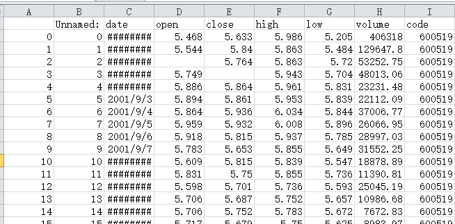
1
2
3
4
5
6
7
8
9
10
11
12
13
14
15
16
17
18
19
20
21
22
23
24
25
26
27
28
29
30
31
32
33
34
35
36
37
38
39
40
41
42
43
44
45
46
47
48
49
50
51
52
53
54
55
56
57
58
59
60
61
62
63
64
65
66
67
68
69
70
71
72
73
74
75
76
77
78
79
80
81
82
83
84
85
86
87
88
89
90
91
92
93
94
95
96
97
98
99
100
101
102
103
104
105
106
107
108
109
# 默认读取一支股票的数据
In [59]: d = pd.read_csv('d.csv')

In [60]: d
Out[60]:
Unnamed: 0 date open close high low volume code
0 0 2001-08-27 5.468 5.633 5.986 5.205 406318.00 600519
1 1 2001-08-28 5.544 5.840 5.863 5.484 129647.79 600519
2 2 2001-08-29 5.859 5.764 5.863 5.720 53252.75 600519
3 3 2001-08-30 5.749 5.878 5.943 5.704 48013.06 600519
4 4 2001-08-31 5.886 5.864 5.961 5.831 23231.48 600519
... ... ... ... ... ... ... ... ...
3876 3876 2017-12-11 631.000 650.990 651.950 631.000 72849.00 600519
3877 3877 2017-12-12 658.700 651.320 658.770 651.020 47889.00 600519
3878 3878 2017-12-13 654.990 668.210 670.000 650.720 48502.00 600519
3879 3879 2017-12-14 669.980 664.550 671.300 660.500 31967.00 600519
3880 3880 2017-12-15 664.000 653.790 667.950 650.780 32255.00 600519

[3881 rows x 8 columns]

# 指定date列为行索引,并转为日期索引
In [73]: d = pd.read_csv('d.csv', index_col='date', parse_dates=True)

In [74]: d.index
Out[74]:
DatetimeIndex(['2001-08-27', '2001-08-28', '2001-08-29', '2001-08-30',
'2001-08-31', '2001-09-03', '2001-09-04', '2001-09-05',
'2001-09-06', '2001-09-07',
...
'2017-12-04', '2017-12-05', '2017-12-06', '2017-12-07',
'2017-12-08', '2017-12-11', '2017-12-12', '2017-12-13',
'2017-12-14', '2017-12-15'],
dtype='datetime64[ns]', name='date', length=3881, freq=None)

# 将date列解析为日期
In [75]: d = pd.read_csv('d.csv', parse_dates=['date'])

In [76]: d.date
Out[76]:
0 2001-08-27
1 2001-08-28
2 2001-08-29
3 2001-08-30
4 2001-08-31
...
3876 2017-12-11
3877 2017-12-12
3878 2017-12-13
3879 2017-12-14
3880 2017-12-15
Name: date, Length: 3881, dtype: datetime64[ns]

# 读取date和open列
In [104]: d = pd.read_csv('d.csv', usecols=['date', 'open'])

In [105]: d
Out[105]:
date open
0 2001-08-27 5.468
1 2001-08-28 5.544
2 2001-08-29 5.859
3 2001-08-30 5.749
4 2001-08-31 5.886
... ... ...
3876 2017-12-11 631.000
3877 2017-12-12 658.700
3878 2017-12-13 654.990
3879 2017-12-14 669.980
3880 2017-12-15 664.000

[3881 rows x 2 columns]

# 跳过文件第一行,设置列索引为abcdefg
In [108]: d = pd.read_csv('d.csv', header=None, skiprows=1, names=list('abcdefg'))

In [109]: d
Out[109]:
a b c d e f g
0 2001-08-27 5.468 5.633 5.986 5.205 406318.00 600519
1 2001-08-28 5.544 5.840 5.863 5.484 129647.79 600519
2 2001-08-29 5.859 5.764 5.863 5.720 53252.75 600519
3 2001-08-30 5.749 5.878 5.943 5.704 48013.06 600519
4 2001-08-31 5.886 5.864 5.961 5.831 23231.48 600519
... ... ... ... ... ... ... ...
3876 2017-12-11 631.000 650.990 651.950 631.000 72849.00 600519
3877 2017-12-12 658.700 651.320 658.770 651.020 47889.00 600519
3878 2017-12-13 654.990 668.210 670.000 650.720 48502.00 600519
3879 2017-12-14 669.980 664.550 671.300 660.500 31967.00 600519
3880 2017-12-15 664.000 653.790 667.950 650.780 32255.00 600519

[3881 rows x 7 columns]

# 指定null和None为缺失值
In [116]: d = pd.read_csv('d.csv', na_values=['null', 'None'])

In [117]: d
Out[117]:
Unnamed: 0 date open close high low volume code
0 0 2001/8/27 5.468 5.633 5.986 5.205 406318.00 600519
1 1 2001/8/28 5.544 5.840 5.863 5.484 129647.79 600519
2 2 2001/8/29 NaN 5.764 5.863 5.720 53252.75 600519
3 3 2001/8/30 5.749 NaN 5.943 5.704 48013.06 600519
4 4 2001/8/31 5.886 5.864 5.961 5.831 23231.48 600519
... ... ... ... ... ... ... ... ...
3876 3876 2017/12/11 631.000 650.990 651.950 631.000 72849.00 600519
3877 3877 2017/12/12 658.700 651.320 658.770 651.020 47889.00 600519
3878 3878 2017/12/13 654.990 668.210 670.000 650.720 48502.00 600519
3879 3879 2017/12/14 669.980 664.550 671.300 660.500 31967.00 600519
3880 3880 2017/12/15 664.000 653.790 667.950 650.780 32255.00 600519

文件写入

写入到csv文件: to_csv函数

写入文件函数的主要参数

  • sep 指定文件分隔符
  • na_rep 指定缺失值转换的字符串,默认为空字符串
  • header=False 不输出列名一行
  • index=False 不输出行索引一列
  • columns 指定输出的列,传入列表

默认写入

1
2
3
4
5
6
7
8
9
10
11
12
13
14
15
16
17
18
In [120]: d
Out[120]:
Unnamed: 0 date open close high low volume code
0 0 2001/8/27 5.468 5.633 5.986 5.205 406318.00 600519
1 1 2001/8/28 5.544 5.840 5.863 5.484 129647.79 600519
2 2 2001/8/29 NaN 5.764 5.863 5.720 53252.75 600519
3 3 2001/8/30 5.749 NaN 5.943 5.704 48013.06 600519
4 4 2001/8/31 5.886 5.864 5.961 5.831 23231.48 600519
... ... ... ... ... ... ... ... ...
3876 3876 2017/12/11 631.000 650.990 651.950 631.000 72849.00 600519
3877 3877 2017/12/12 658.700 651.320 658.770 651.020 47889.00 600519
3878 3878 2017/12/13 654.990 668.210 670.000 650.720 48502.00 600519
3879 3879 2017/12/14 669.980 664.550 671.300 660.500 31967.00 600519
3880 3880 2017/12/15 664.000 653.790 667.950 650.780 32255.00 600519

[3881 rows x 8 columns]

In [121]: d.to_csv('d0.csv')

image-20240108183934591

不输出行索引一列

1
In [123]: d.to_csv('d0.csv', index=False)

image-20240108184058188

行列索引都不写入

1
d.to_csv('d0.csv', index=False, header=False)

image-20240108184200336

仅写入指定列

1
d.to_csv('d0.csv', index=False, columns=['date', 'open'])
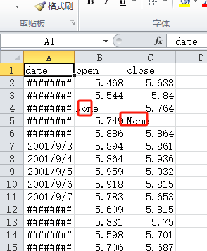
image-20240108184504593

使用指定字符串填充缺失值

1
d.to_csv('d0.csv', index=False,columns=['date', 'open', 'close'], na_rep='None')

image-20240108184757649